How does a bike-share navigate speedy success

•

This is a case study based on a fictional company named Cyclistic bike-share. I will be using Microsoft Excel to prepare data, R programming for data analysis and Tableau for the visualizations.

About the company

In 2016, Cyclistic launched a successful bike-share offering. Since then, the program has grown to a fleet of 5,824 bicycles that are geotracked and locked into a network of 692 stations across Chicago. The bikes can be unlocked from one station and returned to any other station in the system anytime.

Until now, Cyclistic’s marketing strategy relied on building general awareness and appealing to broad consumer segments. One approach that helped make these things possible was the flexibility of its pricing plans: single-ride passes, full-day passes, and annual memberships. Customers who purchase single-ride or full-day passes are referred to as casual riders. Customers who purchase annual memberships are Cyclistic members.

Cyclistic’s finance analysts have concluded that annual members are much more profitable than casual riders. Although the pricing flexibility helps Cyclistic attract more customers, Moreno believes that maximizing the number of annual members will be key to future growth. Rather than creating a marketing campaign that targets all-new customers, Moreno believes there is a solid opportunity to convert casual riders into members. She notes that casual riders are already aware of the Cyclistic program and have chosen Cyclistic for their mobility needs.

Moreno has set a clear goal: Design marketing strategies aimed at converting casual riders into annual members. To do that, however, the team needs to better understand how annual members and casual riders differ, why casual riders would buy a membership, and how digital media could affect their marketing tactics. Moreno and her team are interested in analyzing the Cyclistic historical bike trip data to identify trends.

The following data analysis steps will be followed:

Ask, Prepare, Process, Analyze, Share, Act.

Ask

Key tasks followed.

1. Business task identified.

2. key stakeholders considered.

Business Task: Design marketing strategies aimed at converting casual riders into annual members.

The questions that need to be answered are:

1. How do annual members and casual riders use Cyclistic bikes differently?

2. Why would casual riders buy Cyclistic annual memberships?

3. How can Cyclistic use digital media to influence casual riders to become members?

Key Stakeholders:

· Lily Moreno — Director of the marketing team and my manager.

· Cyclistic executive team

Prepare

Key Tasks Followed:

1. Downloaded data and copies have been stored on the computer.

2. It was downloaded from March 2023 to February 2024

3. The data is in -xls and it has thirteen columns.

4. The data follows the ROCCC .

For the data analysis, it has been downloaded the Cyclistic historical data trips of 12 months, from March 2023 to February 2024 and will be using Microsoft Excel. Dataset

1. The datasets were downloaded and renamed into “year_month-divvy-tripdata” organized in .xls in a folder named 2023_03_to_2024_02.

2. All the datasheets possess the same attributes, the data types are appropriate and consistent; the attributes are ride_id, rideable_type, started_at, ended_at, start_station_name, start_station_id, end_station_name, end_station_id, start_lat, start_lng, end_lat, end_lng and member_casual

3. The dataset follows the ROCCC Analysis as described below: Reliable — it is not biased; Original — the original data can be located; Comprehensive — there is missing information, but it is not important information; Current — it is updated monthly and cited — yes.

4. The “started_at” and “ended_at” columns were changed to the format year_month-divvy-tripdata.

5. The information was separated using split and choosing as delimiter “,” and verifying how decimals are treated in advanced settings.

6. The format of the column “started_at” and “ended_at” was change to “dd/mmm/yyyy hh:mm:ss AM/PM” so it shows date, hour and if it is morning or afternoon.

7. Each column was revised and given a format according to its data.

8. The column width was adjusted with auto adjust column width.

9. The column “ride_length” its crated, it is given the format “HH:MM:SS” and we put the formula to subtract column “started_at” to column “ended_at” like =(D#-C#) to calculate the time wasted in the ride.

10. The column “day_of_week” uses the formula to calculate the day of the week the ride started, so it will throw number from 1 to 7, 1=Monday and 7=Sunday. The formula is “=WEEKDAY(C#)”.

Process

Key Tasks Followed:

1. Data checked for errors.

2. RStudio was chosen as a tool.

3. Data was transformed so we can work it.

4. The cleaning process was documented .

To clean, analyze, and aggregate the large amount of monthly data stored in the folder, we will be using RStudio.

1. Conduct descriptive analysis:

a. We calculate mean ride length with “=AVERAGE(N:N;N1)” and maximum with “=MAX(N:N;N1)”, also mode for day of week with “=MODE(O:O;O1)”.

b. We create a pivot table: rows=member_casual; values=Average of ride_length; columns=day_of_week and values=Count of ride_id. To calculate the average ride length for members and casual riders.

2. We created a new script.

3. We set the work directory.

setwd(“C:/Users/rmoca/OneDrive/Escritorio/Case_April_2024”)

4. We installed the required packages.

install.packages(“tidyverse”)

install.packages(“lubridate”)

install.packages(“janitor”)

install.packages(“readxl”)

install.packages(“writexl”)

5. We loaded the packages.

library(tidyverse)

library(lubridate)

library(janitor)

library(“readxl”)

library(“writexl”)

6. Import data to R frame.

df1 <- read_xlsx(“C:/Users/rmoca/OneDrive/Escritorio/Case_April_2024/cleaned_data/2023_03-divvy-tripdata.xlsx”)

df2 <- read_xlsx(“C:/Users/rmoca/OneDrive/Escritorio/Case_April_2024/cleaned_data/2023_04-divvy-tripdata.xlsx”)

df3 <- read_xlsx(“C:/Users/rmoca/OneDrive/Escritorio/Case_April_2024/cleaned_data/2023_05-divvy-tripdata.xlsx”)

df4 <- read_xlsx(“C:/Users/rmoca/OneDrive/Escritorio/Case_April_2024/cleaned_data/2023_06-divvy-tripdata.xlsx”)

df5 <- read_xlsx(“C:/Users/rmoca/OneDrive/Escritorio/Case_April_2024/cleaned_data/2023_07-divvy-tripdata.xlsx”)

df6 <- read_xlsx(“C:/Users/rmoca/OneDrive/Escritorio/Case_April_2024/cleaned_data/2023_08-divvy-tripdata.xlsx”)

df7 <- read_xlsx(“C:/Users/rmoca/OneDrive/Escritorio/Case_April_2024/cleaned_data/2023_09-divvy-tripdata.xlsx”)

df8 <- read_xlsx(“C:/Users/rmoca/OneDrive/Escritorio/Case_April_2024/cleaned_data/2023_10-divvy-tripdata.xlsx”)

df9 <- read_xlsx(“C:/Users/rmoca/OneDrive/Escritorio/Case_April_2024/cleaned_data/2023_11-divvy-tripdata.xlsx”)

df10 <- read_xlsx(“C:/Users/rmoca/OneDrive/Escritorio/Case_April_2024/cleaned_data/2023_12-divvy-tripdata.xlsx”)

df11 <- read_xlsx(“C:/Users/rmoca/OneDrive/Escritorio/Case_April_2024/cleaned_data/2024_01-divvy-tripdata.xlsx”)

df12 <- read_xlsx(“C:/Users/rmoca/OneDrive/Escritorio/Case_April_2024/cleaned_data/2024_02-divvy-tripdata.xlsx”)

7. Merge all into a data frame.

cyclistsrides <- rbind(df1,df2,df3,df4,df5,df6,df7,df8,df9,df10,df11,df12)

8. See the dimensions of the new data frame.

dim(cyclistsrides)

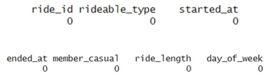
9. Check for these columns if there is any NA value: “ride_id”, “rideable_type”, “started_at”, “ended_at”, “member_casual”, “ride_length” and “day_of_week”. That is considered relevant data.

colSums(is.na(cyclistsrides[,c(“ride_id”, “rideable_type”, “started_at”, “ended_at”, “member_casual”, “ride_length”, “day_of_week”)]))

10. We check that “ride_length” have NA values, after checking we conclude that those values where track errors of time: for example, rider id 123456 starts at starting point at 01:30 PM on the 01/mar/2023 and he arrives at ending point at 1:10 PM on the 01/mar/2023.

So those values are irrelevant to the data frame.

11. Clear NA values for “ride_length”.

cyclistsrides<-cyclistsrides[!(is.na(cyclistsrides$ride_length)), ]

12. Verify if there is any NA value after cleaning.

colSums(is.na(cyclistsrides[,c(“ride_id”, “rideable_type”, “started_at”, “ended_at”, “member_casual”,”ride_length”,”day_of_week”)]))

13. Check if there is any duplicated trip, so we are checking only the columns: “ride_id”, “started_at” and “ended_at”.

any(duplicated(cyclistsrides[,c(“ride_id”, “started_at”, “ended_at”)]))

14. There is no duplicate, so we continue with the process.

15. Check the dimensions of the cleaned data.

dim(cyclistsrides)

16. Check the structure of the new data frame.

str(cyclistsrides)

17. Save the data frame.

write.csv(cyclistsrides, “2023_03–2024_02.csv”)

Analyze

Key tasks followed:

1.Data was aggregated.

2. Data was organized and formatted.

3. Calculations were performed.

4.Trends and relationships were identified.

1. Check the mean length ride.

mean(cyclistsrides$ride_length)

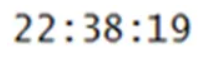
2. Check the maximum length ride.

max(cyclistsrides$ride_length)

3. Obtain the trip duration per day and per bike.

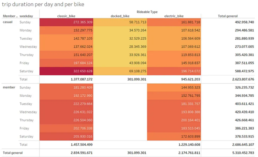
Casual users use more the service during weekends while member users from Tuesday to Thursday.

Both use more of the classic bike.

4. Compare casual vs member users and which type of bike they use.

We can see that member users are the majority in classic and electric bikes, and that casual users are the only ones that use docked bikes.

5. Obtain the average ride and number of rides per day of the week.

We can see that casual users use more the service during weekends and make more large trips also during weekends.

But member users use more the service during the week, but the longest trips are during weekends.

6. Obtain the average ride and number of rides per month.

We can see that both users use less the service during cold months (probably because of chilly weather) and have the shortest rides, except for the second month of the year.

7. Obtain the average ride and number of rides per year.

We can see that there is a decrease and that casual users use more the service and take the longest rides.

8. Obtain ride trends by hour of usage.

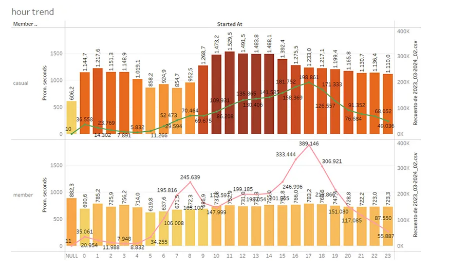
We can see that casual and member users use the service during office hours and that the peak is from 4 pm to 7 pm.

Also, that member users have the same ride length during the day while the longest rides of casual users are during lunch hours.

The graphs used can be viewed from my tableau.

You can check my portfolio.

Act

Recommendations

To convert casual riders into annual members, the following marketing strategies can be implemented:

We can provide discounts or a special plan to casual members;

- During summer.

- On weekends.

- During lunch hours.

We can also increase the rental on those moments for casual members, so they have an incentive or reason to become members.

R Code

# code to process data

# install the required packages